This post summarises the essential steps in putting together a survey-grade GNSS unit using the LC29HDA from Quectel for a very modest financial outlay; a single LC29HDA module with a good quality antenna was bought for a little over £40 (they were on offer. This was found to give repeatable positioning to only a few cm.
This is not a full tutorial but it should be fairly easy to find background information on GNSS and RTK (although I found this e-book to be a good guide to some of the theory and practice), and for Bluetooth and LoRa. I will not repeat what can be easily found on the web or in datasheets. I will, however, provide some “beginner level” information where I consider this is helpful in allowing readers to do their own background reading, as it is sometimes hard to work out what is relevant.
For some initial background reading: look up what the difference between GNSS and GPS is (even though we colloquially use GPS when we should say GNSS); find out what “rover” and “base” mean in the context of RTK.
Two Aims
There are essentially two ways of getting a survey-grade position using RTK: using a third party base station and the NTRIP protocol over the internet, or running your own base station and feeding the RTCM messages direct into the rover. The first case will be find if there is a nearby (typically <30km) accessible third party base station and a strong enough “mobile data” signal at the survey location. My setup for this is an Android phone with SWMaps and a connection to the GNSS unit using Bluetooth. The second case is for if the first does not apply. My setup for this uses the LoRa radio technology to communicate RTCM messages from the base station direct to the rover GNSS unit (still connected to the phone via Bluetooth). More on the detailed setups later!
The LC29HDA can be configured to work as a base and as a rover (in spite of what some sites say, the base station does not requie purchase of a LC29HBS).
Preparations
This is aimed at the beginners. There are three things to consider to avoid looking at your shiny GNSS module and saying “what next?”: electrical connection, communication with your PC, and powering. A bit of soldering will also be required.
Electrical Connection
You could use solderless breadboard if you have it but I often use what tend to be called “DuPont” connectors. These are 0.1″ pitch connectors which are widely available in both double-ended sockets and socket-to-pin versions.
Powering
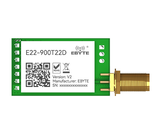
You need to be a bit careful with voltages as the communications (see below) for the modules in question is at 3.3V but the boards used are powered by more than 3.3V and have a voltage regulator on-board (top right in the LC29HDA module pictured below) which converts the supply to what the inner electronics requires. The ability to power the modules with higher voltages is helpful in that it allows us to use something like a “power bank” (5V, typically used for mobile phone charging) or a 18650 Lithium cell (working voltage about 3.7V, max voltage about 4.2V). My preferred option is to use 18650 Lithium cells; these are rechargeable, readily available (being used in “vaping” devices), are available in sufficiently high capacities, and you can get battery holders for them. Beware, though, that there are LOTS of people selling cheap 18650 cells which do not have the advertised capacity and may not have sensible safety devices inside; I always get mine from a specialist seller or a proper electronics retailer such as CPC.
PC Communications
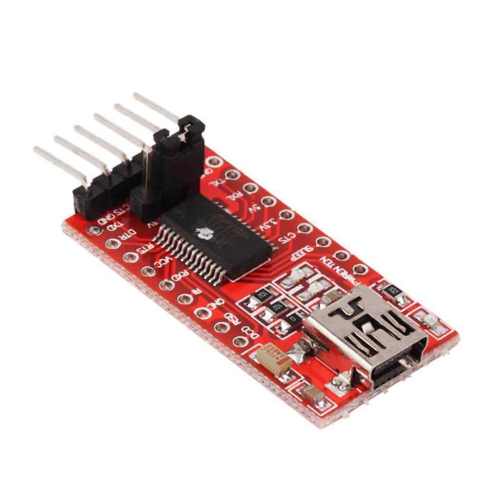
The modules communicate using a digital protocol known as UART, which uses a series of pulses to encode the binary format of the messages. We don’t need to worry about this level of detail, other than to be sure that the voltage of the pulses matches, when connecting modules together (which they do for the modules I mention). In order to communicate between a PC and modules, we need an adapter that can convert between the UART digital signals and appear as a USB serial port (a “COM” port on Windows). We also need some software to display what is received on the serial port, and to allow us to send messages. The software I tend to use is called Termite but there are plenty of options for Windows, MacOS, and linux, and plenty of guides on the web to choosing and using serial terminal software. Similarly, there are plenty of guides to connecting the adapters (the most important thing is to connect the TX from the module to the RX of the adapter and vice versa, noting that TX=transmit means data coming out of the connector).
There are several options for the UART to USB serial adapter, but consideration has to be given to the communication voltage (or risk burning out your module!). Some of these have a removable jumper to change the voltage from 3.3V to 5V, while others have a “solder jumper”.
One option is to power the module from a battery and to only connect the ground (0V), RX and TX of the adapter.
The other option is to use the adapter to provide power to the module. This is where care is required because if you set the adapter to use 3.3V logic then its Vcc pin will be at 3.3V and this may not be sufficient to properly power the module (recall that these have a voltage regulator on board which will “drop” some voltage, leaving the module potentially under-powered). There is also the issue that the maxiumum current which the 3.3V supply from the adapter board can support may be less than the module(s) require; the LC29HDA peaks at about 100mA.
My preferred option is to use a FTDI232 serial adapter board with a jumper set to the 3.3V position and to plug a DuPont connector onto the bare pin next to the jumper, as this should be at 5V (check your adapter!). There are currently boards on the market with solderable holes on the sides which can also be used to access the 5V supplied by the USB connector (I suspect many of these use clone FDTI232 chips, but they probably work fine). The 5V supply from the USB port should be good to 500mA, plenty for our uses.
LC29HDA GNSS Modules and Antennas
Note that there are several very different models which start “LC29H”. The DA supports RTK at an update frequency of 1Hz, which is fine for survey use, while another model gives 10Hz for use cases such as drones. Some models do not support RTK at all. These are dual frequency band (L1 + L5) devices, which is important for high accuracy. Note that this is different to being multi-constellation (which they are), which means they can use satellites from GPS, GLONASS, Galileo, BeiDou, etc systems.
The Quectel website has several brochures and data sheets to refer to. You will also need the “protocol specification”, which describes the messages which can be sent to/from the LC29H (although most will not be directly relevant), and I recommend using their QGNSS software.
I bought a module and the more expensive antenna (probably a Quectel YB0017AA, although it is not branded) from Panda Wireless on Aliexpress (note that the picture is from their listing and is for the EA variant, also that the antenna is actually ~6cm square and the LC29HDA board is 3cm long). Ensure you use a dual band L1 + L5 antenna. The YB0017AA is claimed to be IP65 rated so should be weather-proof in all reasonable conditions. Panda wireless were attentive and clearly wanted to be sure that I knew what I was doing; I suspect they have had too many returns from people who did not!
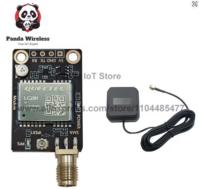
The board has a backup battery (top left in image) which is rechargeable but will only work if the module is powered for quite some time (at least 1 day?). This will allow the GNSS to more quickly get a fix if powered down for up to a few hours. A “cold start” needs about 30s to get a position fix.
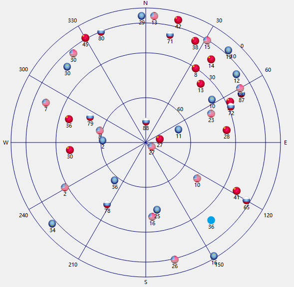
At this point, connect the antenna (ideally place it outside) and the LC29HDA module to your serial adapter (TX/RX cross-over) and connect to your PC. It will take about 30s for a position fix after which the green PPS LED will flash. Set QGNSS to refer to the serial port associated with the adapter, using a 115200 baud connection speed (the default for LC29H) and explore the features of QGNSS.
Once you’ve explored the graphical presentation of position and GNSS performance, take a look at the data/messages coming out of the module. There are several viewers under the “View” menu but I found the most useful was the Console tool (“Tools” menu) because the module emits lots of messages every second. Use the “Message Statistics” tab and move the splitter (two short vertical bars) leftwards. This allows you to home in on a particular message type and see its latest contents decoded.
Now would be a good time to look up the format of NMEA messages and to consult the protocol specification document to correlate the explanations with the messages coming out of the GNSS module.
As an extra, try using Termite (or alternative) to connect and see the messages. You will need to set it to 115200 baud (and the default of 8 data bits, no parity and 1 stop bit). Be sure to disconnect QGNSS first; only one program can use a serial port at a given time.
Concerning Firmware
The firmware is the software program running inside the LC29HDA. The version is shown at the bottom of QGNSS and the modules supplied to me had version LC29HDANR11A03S_RSA. This works fine but does not have the NMEA GST message which contains information about the location accuracy. I contacted Quectel who provided me with LC29HDANR11A04S_RSA, which does. The firmware can be updated using QGNSS. During this process, QGNSS says you should reset the module by pressing a button! All you need to do is to briefly disconnect power from the LC29HDA (leaving the serial adapter connected to the PC).
Using NTRIP for RTK
Since the default mode for the LC29HDA is to function as a rover, all we need to do now is to acquire NTRIP data from a server and use it to generate RTCM3 messages to send to the GNSS module. QGNSS can do this; see under the Tools menu.
There are plenty of commercial NTRIP services but RTK2Go has a public “NTRIP Caster” and quite a few people who send their base station data to the RTK2Go server for distribution to anyone for free. A map of base stations allows you to see if there is once close enough (as a rough guide, a base station closer than ~10km should give you ~2cm level fixes and over 30km might struggle to get a fix, depending on conditions. My nearest station is called WEBBPARTNERS so in the QGNSS NTRIP Client setting I provide “rtk2go.com”, “2101” for the port, and my email address as the username (no password needed for client access). Then just “Update NTRIP Source Table” and choose the nearest station then “Connect to Host”.
Initially, the fix quality will appear as “RTK Float”, while the algorithm is working out position ambiguities, but after a while it will show a “RTK Fix”.
NB: for RTK to be able to get a “fix”, the antenna must have a good wide view of sky. A window cill is likely to be no good.
Bluetooth
Although it would be possible to make a wired connection via USB to a phone/tablet, it seems quite an ugly approach, and Bluetooth is the obvious contender. What we need here is something equivalent to the UART serial to USB adapter but with a wireless link in the middle. So the bluetooth module needs to speak UART to communicate with the GNSS module and the Bluetooth messages need to be interpreted as serial communications on the phone/tablet/PC. We need a Bluetooth-serial module.
My preferred software, SWMaps. supports both Bluetooth Classic and Bluetooth Low Energy (BLE). Initial trials with BLE were not successful as the NMEA messages got truncated and overlapped by the time they were passed to SWMaps. I believe this is probably down to the BLE modules I tested being v4.0 (most cheap modules use this version) and having too short a message size (20 bytes) to transfer the GNSS output at the programmed BLE connection rate. It was possible to reduce the message truncation by dropping the GNSS baud rate but the LC29H documentation recommends 115200 baud and is was clear from experiments that there is an unavoidable bottle-neck. Rather than investigate BLE v5.0 (or v4.2) modules I opted to go the Bluetooth Classic route. This also means that Windows 11 can connect via Bluetooth too*; once connected, another serial port will appear (actually usually two appear, only one of which works!!). If you use iOS I understand you will have to use BLE.
[* – this may be a hardware issue but I consistently failed to be able to connect a BLE serial device, although I believe BLE audio may be possible]
The HC-06 and HC-05 modules are well known and have been available for several years. These should be Bluetooth Classic but some suppliers are selling devices they describe as HC-06/05 which are actually BLE (only). BLE and Bluetooth Classic are not at all interoperable. Recent purchases of HC-05/6 have been also bad, even when they were Bluetooth Classic; whereas my 10 year old module worked fine with the NTRIP->RTCM relay (see below), recent items claiming to be HC-06 with LINVOR 1.8 firmware simply crashed when attempting to send these messages to the GNSS while receiving the NMEA location data.
I ended up using the slightly less popular JDY-31 modules on a carrier board which allows for a 3.6V-6V power supply but have a 3.3V logic level (see earlier). We do not need “EN” and “STATE”, so a 4 pin device will be fine. Bare modules that have outlines like a postage stamp won’t do. These worked without issue. They also advertise a BLE service, but without a device name; this is not connectable with most Android apps (but it was with nRF Connect) or from Windows, but maybe you iOS users can make it play…
Search the web for more information on the JDY-31, especially the “AT Commands” which are used to configure the module.
Connect the JDY-31 to your USB serial adapter, crossing over TX/RX. Establish a connection using Termite with a baud rate of 9600 (which should be the supplied default). NB: this is not connecting via Bluetooth, but by the USB connection.
For some basic testing, you can either make a Bluetooth connection from your PC (probably you have to buy an adapter for a destop) and then run a second instance of Termite, or install a suitable app on your phone. Suitable apps on Android include Bluetooth Serial Monitor by ArduinoGetStarted or Serial Bluetooth by Kai Morich. These both support both BLE and Bluetooth Classic and so can be used to check your BT module is kosher or not.
Once the BT module is connected to your PC/phone (LED should go permanently on, a PIN of 1234 is usually required), it should be possible to send text messages from Termite to the app (or other Termite window).
To prepare the BT module for use with the GNSS, first disconnect the BT, leaving just the USB serial adapter as the means of communication and use the AT+BAUD command to change the baud rate to 115200 (you may have to issue an AT+RESET to make this take effect). If it works you’ll then have to change Termite to use 115200 too. Maybe also change the module name and decide whether you want a different PIN.
Remove the USB serial adapter and connect the GNSS module to the BT module, with a shared power supply (battery) and RX/TX crossover. You should now be able to connect to the BT module and view the NMEA messages on your phone/PC along the lines noted above. On a PC it should be possible to use QGNSS after setting it to use the serial port associated with the BT connection.
It should now be straight-forward to make a connection via Bluetooth from SWMaps (or whatever), noting that only one connection at a time is possible. The default configuration of the LC29HDA modules causes almost all of the NMEA messages which SWMaps can use; it does not emit the GST message (see above, under firmware). For different mapping or logging software you might find there are different requirements; check the documentation and compare to the NMEA messages summarised in the QGNSS Console.
The GST messages can be enabled, given the right firmware, by using the $PQTMCFGMSGRATE command in the GNSS Console (Message Statistics tab). The command is:
$PQTMCFGMSGRATE,W,GST,1*0B
To make this apply after a power cycle, save the setting using:
$PQTMSAVEPAR*5A
The part following the “*” is the checksum and QGNSS Console will helpfully generate it for you. Do some background reading on the checksum.
Using NTRIP for RTK Revisited
This was already described for QGNSS but it is now a snip to turn into a mobile station; all we need to do now is to set SWMaps (or whatever) to acquire NTRIP data using the same information as previously, which it then converts to RTCM3 messages and sends over the BT connection to the GNSS module.
The first of the two aims is now satisfied. Magic! See later in this post for a short account of a basic performance trial.
LoRa – Radio Link for Base Station
There are lots of options for making the wireless connection from a base station to the rover, with the essential requirement being something which can translate our UART in/out messages to a wireless protocol. I used LoRa, specifically the E22 modules from Ebyte because I’d already experimented with them and been impressed by the signal range, ability to cope with non-clear line of sight, ease of use, and price. The E22 modules are available in different frequency bands, not all of which are licenced in all regions. The 868MHz band is probably the best for Europe. Two modules will be required, of course, but buying an extra one with a built-in USB adapter does make exploring/testing easier.
In addition to the frequency band, the E22 module is available with different powers and connection arrangements. The higher powers are thought to not be legal in the UK (do your homework!). I suggest the E22-900T22D (and buy an antenna of the correct frequency band too).
 EByte provides adequate documentation and a software configuration tool, which makes setting the modules up easier. See the documentation for how to use the M0/M1 pins to put the module into configuration mode. Here are the settings for the rover:
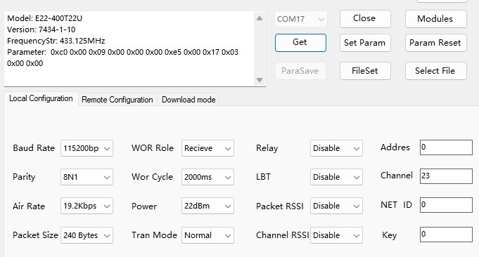 Note that the baud rate is set to match the GNSS module and that I have chosen an air data rate of 19200 baud. The default air rate of 2400 baud gives about 5km range but is too slow for the spew of RTCM messages which must be communicated. The higher data rate will give a smaller range, but hopefully sufficient. The rover and base station must use the same air data rate, channel and “net id”. I have set the rover address to be 0, whereas for the base station this MUST be 65535 (this is the FFFF hexadecimal address), which is required for the messages to be broadcast – see the E22 documentation.
Once configured, connect both M0 and M1 pins to 0V/ground to put the module into “transparent” mode. Connect the USB serial adapter to one E22, noting that these modules are intended to be powered by 5V supply* but have 3.3V UART logic. Use an E22-900T22U or a second USB serial adapter to make up the other end of the LoRa data link, open two Termite windows and connect them to each end, and exchange a few messages.
[* – the datasheet indicates >=5V for good output power, but I have found that a 3.7V 18650 Lithium cell is not noticeably worse in terms of practical range]
Configuring a LC29HDA Base Station
This entails issuing a number of commands using the QGNSS Console (Message Statistics) window and performing module restarts at appropriate points. I did not find a way to initiate an elegant restart, so resorted to briefly disconnecting the power supply to the GNSS module (while leaving the serial adapter connected, in order to avoid dropping the serial connection, although this is just a nuisance).
Change the mode to be a base station then save the change (otherwise it only lasts until a power cycle). Restart the module after these two commands:
$PQTMCFGRCVRMODE,W,2*29
$PQTMSAVEPAR*5A
You should now see that the Console is showing only RTCM messages and no longer NMEA messages. Several different types of message are seen, reflecting the range of satellite constellations; refer to RTCM message documentation to see what they are.
The essential next step is for the base station to know where it is. To do this, the $PQTMCFGSVIN command is used with an a-priori known location or the GNSS module can determine its location by gathering position data for a long period of time; the protocol specification document recommends 12 hours! Since we’re mostly not going to know a precise location, the automatic “survey-in” procedure is likely to be the way to go. Additionally, if we don’t need the absolute position accuracy to be at the cm level, a shorter automatic survey-in period might be acceptable. For example, if we get to 10cm accuracy and: a) record and re-use the same geospatial position and the determined coordinates, and b) before each survey session record the location of a few well-defined/documented points, we should have good cm-level relative accuracy within the survey and enough information for a later adjustment to absolute accuracy, if required. Top quality absolute accuracy is also going to require consideration of datums and epochs which take account of continental drift, for example. This is not in scope for this post!
For the purpose of testing/demonstration, a survey-in period of 2 minutes is a reasonable starting point. With a moderately good sky view I got a 0.25m accuracy estimated by the GNSS in only 60s. To monitor the progress of the survey-in process, we should first enable the $PQTMSVINSTATUS messages (see the protocol specification). The set of messages to send to the GNSS module is:
$PQTMCFGMSGRATE,W,PQTMSVINSTATUS,1,1*58
$PQTMCFGSVIN,W,1,120,0,0,0,0*21
$PQTMSAVEPAR*5A
Then restart the module and observe the $PQTMSVINSTATUS messages in the Console (Protocol Package). Once the GNSS has got a position fix, the PQTMSVINSTATUS messages should start to change and continue to do so for as long as the survey in period (120s in the command above). Watch the accuracy improve and the status message finally show valid=2.
Connecting the Base and Rover
The second aim is now in sight!
A trial run without involving the LoRa radio link can be attempted by making a wire connection between the base and rover. The TX output from the base should be connected to the RX input of the rover (and any other connection to the rover RX removed). It is still OK to have either a USB serial adapter or BT adapter connected to the rover TX (only) and this can be used to establish a connection from QGNSS to the rover to see it get the RTK Fix, at which time the variation of the location seen via the “Deviation Map” will suddenly drop to a few cm.
The final step is to replace the wire with a LoRa link. The rover GNSS should have its TX connected to the BT RX – this will send the NMEA messages out over Bluetooth. The rover RX should be connected to the TX of the E22 module with address = 0. This is how it gets the RTCM RTK messages. The base station GNSS TX should be connectd to the RX of the E22 module with address 65535 (FFFF hex). The base station will probably also need either another BT module or a USB serial adapter connected so that the survey-in command can be sent (and survey-in process monitored via the $PQTMSVINSTATUS messages). It is OK for the base station GNSS TX to be connected to both LoRa E22 RX and USB serial adapter RX. Use separate power sources for each of the rover and base.
Set the base station up somewhere and do not move it, connect your phone to the rover via Bluetooth, watch the RTK Fix be established… and be amazed. This is truely awesome technology!
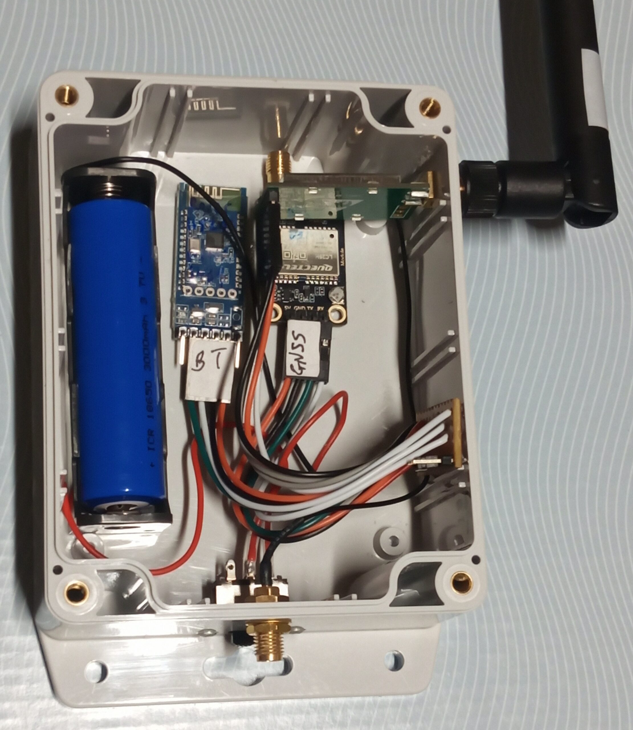
The Finished Rover
NTRIP for RTK Basic Performance Trial
This was done from my garden which has a nearby buildings and trees. I’m using the WEBPARTNERS source of correction data from rtk2go.com, which is about 25km distant. Overall, this seems like a reasonable real-world-imperfect test case.
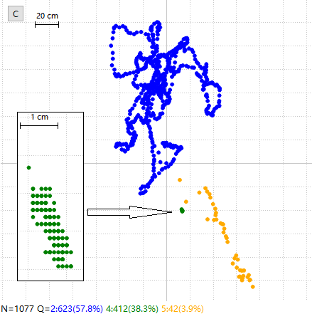
Although no absolute location data is known to compare the reported “green dot” positions to a ground truth, it is quite clear that even a quick survey with DGNSS alone is going to have quite distorted dimensions for features of the order of a few 10s of metres, as the GNSS location wanders about during the survey, ie poor relative accuracy. The RTK results compete with someone using a tape measure.